Cluster Monte Carlo for the Ising Model

From a problem set in my first-year computational physics course (G6080).

The two-dimensional Ising model assigns a spin $\sigma_i = \pm 1$ to every site of a square lattice, with the energy (in units where $k_B T = 1$) written as

$$E = -J \sum_{\langle ij \rangle} \sigma_i \sigma_j$$

where the sum runs over nearest-neighbor pairs and $J$ is the coupling. Onsager solved this model exactly, and the phase transition sits at $J_c = \tfrac{1}{2}\ln(1 + \sqrt{2}) \approx 0.4407$. Below that coupling the lattice is a disordered salt-and-pepper mess, and above it one spin orientation wins. Sampling this model is the classic playground for Monte Carlo, and also where the simplest Monte Carlo fails.

Critical slowing down

The textbook Metropolis algorithm flips one spin at a time. Near the critical point that becomes agonizing, because the system organizes into correlated patches whose size is set by the correlation length, and flipping one spin inside a patch does almost nothing. The random walk through configuration space stalls, and the autocorrelation time blows up as the correlation length grows.

Cluster algorithms attack the patches directly. The Wolff single-cluster algorithm picks a random seed spin and grows a cluster outward from it. Each aligned nearest neighbor joins the cluster with probability

$$p = 1 - e^{-2J}$$

and once the cluster stops growing, every spin in it flips at once. That particular acceptance probability is chosen such that the whole cluster move is rejection-free while preserving detailed balance, and the algorithm samples the same Boltzmann distribution as Metropolis while moving through configuration space one correlated patch at a time.

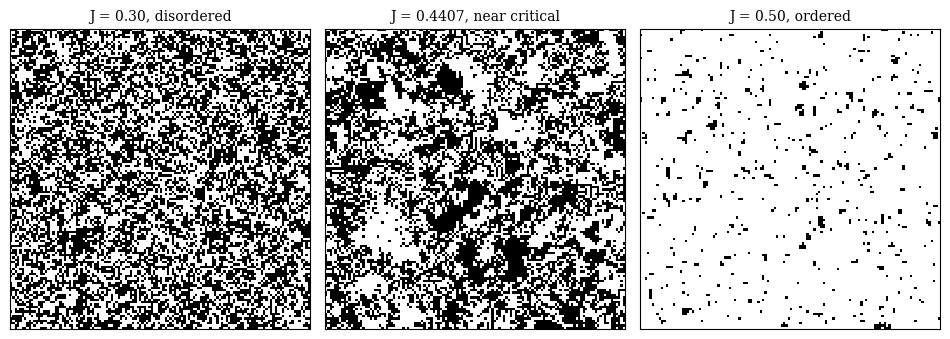
The snapshots above (regenerated from the same algorithm for this note) show the three regimes at a glance. At $J = 0.30$ the lattice is noise. At $J = 0.50$ it is nearly uniform with thermal speckle. Near $J_c$ the configuration has structure on every scale, patches inside patches, which is the regime where single-spin flips stall and cluster flips help most.

Magnetization

Running the cluster algorithm on a $64 \times 64$ lattice at $J = 0.455$, above the transition, the magnetization per spin settles around $\pm 0.9$ but keeps jumping between the two signs, because a large enough cluster flip carries the whole lattice from one ordered phase to the other. A single-spin algorithm at this coupling would stay trapped in one phase for astronomically many sweeps, while the cluster algorithm visits both phases freely, and the physical answer lives in the average of $|M|$.

Correlation length

Above the critical temperature the spin-spin correlation decays exponentially, and on a finite periodic lattice of side $L$ the row-averaged correlation is fit by

$$\langle \sigma(0)\,\sigma(z) \rangle \approx a\left(e^{-z/\xi} + e^{-(L-z)/\xi}\right)$$

where the second term accounts for the periodic image and $\xi$ is the correlation length. The physics says $\xi$ should grow as $J$ approaches $J_c$ from below. My fits at $J = 0.425$, $0.430$, and $0.435$ on a $32 \times 32$ lattice returned correlation lengths far larger than the box itself, and the trend across the three couplings came out scrambled. With only ten measurements per coupling and a correlation length pressing against the lattice size, the fit is dominated by noise and finite-size effects rather than physics. I am leaving that in as recorded, because it is the honest lesson of the exercise. Near a critical point the correlation length is the quantity you want, and it is also the quantity your finite box and finite statistics are least equipped to give you.

Feel free to contact me if there is an error or confusion!