Quantum Tunneling

Inspired by the quantum tunneling series at physicspython.wordpress.com.

Roll a ball at a hill with less energy than it takes to reach the top, and the ball always comes back. Send a quantum wavepacket at a barrier taller than its energy, and some of it shows up on the other side. Let’s watch that happen, and then build the simulation that produced it.

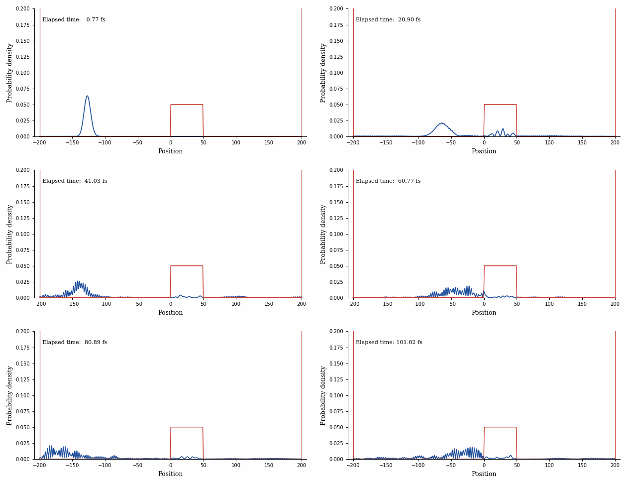
The blue curve is the probability density of the particle, and the red rectangle is the barrier (drawn at a tenth of its height so it fits on the plot). Notice the ripples that appear when the packet reaches the wall. The incoming and reflected waves overlap and interfere, which is something a bouncing ball would never do. Most of the packet comes back, but watch the region inside and beyond the barrier closely. A small piece leaks through and keeps going. That piece is the tunneling.

Setting up the problem

We work in units where $\hbar = m = 1$. The particle starts as a Gaussian wavepacket centered at $x_0$ with width $\sigma$, given a push to the right by the plane-wave factor $e^{ik_0x}$,

$$\psi(x, 0) = (2\pi\sigma^2)^{-1/4}\, e^{-(x - x_0)^2/4\sigma^2}\, e^{ik_0 x}$$

The mean momentum is $k_0$, so the mean kinetic energy is $k_0^2/2$. In the animation $k_0 = 1$ and the barrier height is $V_0 = 0.5$, which puts the packet’s energy right at the top of the barrier. Even so, most of it reflects. The barrier is wide (50 length units against a de Broglie wavelength of $2\pi/k_0 \approx 6$), and a wide barrier suppresses transmission severely.

The packet then evolves under the time-dependent Schrödinger equation

$$i\,\frac{\partial \psi}{\partial t} = \hat H \psi, \qquad \hat H = -\frac{1}{2}\frac{\partial^2}{\partial x^2} + V(x)$$

with $V(x) = V_0$ inside the barrier and zero outside.

Putting it on a grid

A computer cannot hold a continuous function, so we sample $\psi$ at $N$ evenly spaced points and turn $\hat H$ into a matrix. The second derivative becomes the familiar three-point finite difference (think back to the limit definition of a derivative, applied twice),

$$\psi''(x_j) \approx \frac{\psi_{j+1} - 2\psi_j + \psi_{j-1}}{\Delta x^2}$$

which makes $\hat H$ a tridiagonal matrix. The diagonal holds $1/\Delta x^2 + V(x_j)$ and the two off-diagonals hold $-1/2\Delta x^2$. The animation uses 500 points on the interval $[-200, 200]$.

Time evolution

How do we step $\psi$ forward in time? The obvious move is to replace the time derivative by a forward difference and write $\psi^{n+1} = (I - i\,\Delta t\, H)\,\psi^n$. Try it, and the wavefunction grows without bound. The operator $(I - i\,\Delta t\, H)$ is not unitary. Every step therefore inflates the norm a little, and the error compounds over many steps. The fix is the Crank-Nicolson scheme, which treats the step half explicitly and half implicitly,

$$\left(I + \tfrac{i\,\Delta t}{2} H\right)\psi^{n+1} = \left(I - \tfrac{i\,\Delta t}{2} H\right)\psi^{n}$$

The combined one-step operator is unitary (it is the Cayley form of $e^{-iH\Delta t}$), so the norm is preserved to machine precision no matter how long we run. Each frame of the animation is a handful of these steps, with the elapsed time converted to femtoseconds through the atomic unit of time, $2.419 \times 10^{-2}$ fs.

A caveat about the red vertical lines at the edges. The grid ends there, and the wavefunction is pinned to zero at the boundary, which acts like an infinitely hard wall. Run the simulation long enough and the reflected packet bounces off the left wall and comes back for another round. The walls are an artifact of the finite grid, which is why the animation stops before the packet reaches them.

Feel free to contact me if there is an error or confusion!